ML DNN, ANN

Note for Neural Networks (2)

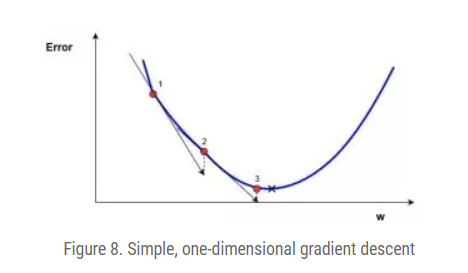
Gradient descent

reduce the error between the anticipated and realistic output

$w_{new}=w_{old}-\alpha*\nabla error$ Here $w_{new}$ denotes the new $w$ position, $w_{old}$ denotes the current or old $w$ position, $\nabla error$ is the gradient of the error at $w_{old}$ and $\alpha$ is the step size.

Example gradient descent (original function after gradient is $4x^3 - 9x^2$):

x_old = 0
x_new = 6
gamma = 0.01
precision = 0.00001


def df(x):
    y = 4 * x ** 3 - 9 * x ** 2
    return y


while abs(x_new - x_old) > precision:
    x_old = x_new
    x_new += -gamma * df(x_old)

print("The local minimum occurs at %f" % x_new)

The cost function :

The cost function for a training pair $(x^z, y^z)$ in a neural network is: $J(w, b, x^z, y^z) = \frac{1}{2}||y^z-h^{(nl)}(x^z)||^2 = \frac{1}{2}||y^z-h_{pred}(x^z)||^2$ This is the cost function of the $z_{th}$ sample where $h^{(n_l)}$ is the output of the final layer

The total cost is: $J_{total}(w, b, x, y) = \frac{1}{m}\sum_{z=0}^{m}\frac{1}{2}||y^z-h^{(nl)}(x^z)||^2 = \frac{1}{m}\sum_{z=0}^{m}J(W, b, x^{z}, y^{z})$ Gradient descent in neural networks $w_{ij}^{(l)} = w_{ij}^{(l)} - \partial\frac{\partial}{\partial w_{ij}^{(l)}}J_{total}(w, b, x, y)$

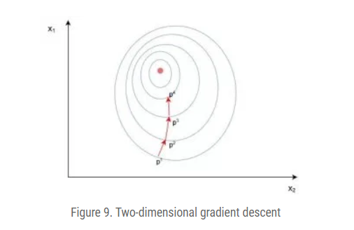
Two dimensional Gradient Descent

Backpropagation in depth (Math Part.)

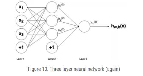
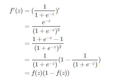
The output of the NN: $h_{w, b}(x) = h_1^{(3)} = f(w_{11}^{(2)}h_1^{(2)}+w_{12}^{(2)}h_2^{(2)}+w_{13}^{(2)}h_3^{(2)}+b_1^{(2)})$ Simplify $h_1^{(3)} = f(z_1^{(2))})$ by defining $z_1^{(2)}$ as: $z_1^{(2)}=w_{11}^{(2)}h_1^{(2)}+w_{12}^{(2)}h_2^{(2)}+w_{13}^{(2)}h_3^{(2)}+b_1^{(2)}$ Then apply gradient descent, we need to calculate the gradient, take the $w_{12}^{(2)}$ as an example $\frac{\partial J}{\partial w_{12}^{(2)}} = \frac{\partial J}{\partial h_1^{(3)}}\frac{\partial h_1^{(3)}}{\partial z_{1}^{(2)}}\frac{\partial z_{1}^{(2)}}{\partial w_{12}^{(2)}}$ Start with the last term $\frac{\partial z_{1}^{(2)}}{\partial w_{12}^{(2)}} = \frac{\partial}{\partial w_{12}^{(2)}}(w_{11}^{(2)}h_1^{(2)}+w_{12}^{(2)}h_2^{(2)}+w_{13}^{(2)}h_3^{(2)}+b_1^{(2)}) \\ = \frac{\partial}{\partial w_{12}^{(2)}}(w_{12}^{(2)}h_2^{(2)}) \\ = h_2^{(2)}$ Then the second term $\frac{\partial h_1^{(3)}}{\partial z_{1}^{(2)}}= f'(z_{1}^{(2)}) = f(z_{1}^{(2)})(1 - f(z_{1}^{(2)}))$ The derivative of sigmoid is

The loss function $J = \frac{1}{2}||y_1-h_1^{(3)}(z_1^{(2)})||^2$ Let $u=||y_1-h_1^{(3)}(z_1^{(2)})||$ and $J=\frac{1}{2}u^2$

Using $\frac{\partial J}{\partial h} = \frac{\partial J}{\partial u}\frac{\partial u}{\partial h}$ $\frac{\partial J}{\partial h} = -(y_1-h_1^{(3)})$ Induce another token $\delta_i^{n_l} = -(y_i - h_i^{(n_l)})·f'(z_i^{(n_l)})$ Then the derivative can be conclude as $\frac{\partial}{\partial w_{ij}^{(l)}}J(w, b, x, y) = h_j^{(l)}\delta_i^{(l+1)}$

Vectorization of backpropagation $\frac{\partial}{\partial W^{(l)}}J(w, b, x, y) = h^{(l)}\delta^{(l+1)}$

$s_l$ is the number of nodes in layer $l$ $\delta^{(l+1)}(h^{(l)})^{T} = (s_{l+1} \times 1) \times (1 \times s_l) = (s_{l+1} \times s_l)$

where ∙ symbol in the above designates an element-by-element multiplication (called the Hadamard product), not a matrix multiplication.

Reference:

[1]. https://adventuresinmachinelearning.com/neural-networks-tutorial/